1.Quantiles, Percentiles, Box Plot
Table of contents
- Quantiles
- Percentile
- 75th percentile usecase
- Box plot
Understanding Quantiles: A Guide to Quartiles, Deciles, Percentiles, and Quintiles
When analyzing data, quantiles help us break data into equal parts. Quantiles divide a dataset into intervals, each containing an equal number of data points.
What Are Quantiles?
Quantiles are cut points in your data that divide it into equal-sized intervals. Depending on the type of quantile, you can divide data into:
- 4 parts (Quartiles)
- 5 parts (Quintiles)
- 10 parts (Deciles)
- 100 parts (Percentiles)
Types of Quantiles
Let’s break down each type of quantile and how it's calculated.
A. Quartiles (Divides Data into 4 Equal Parts)
Quartiles split data into four equal parts. The three quartiles are:
- Q1 (25th percentile): 25% of the data is below this point.
- Q2 (50th percentile or median): 50% of the data is below this point.
- Q3 (75th percentile): 75% of the data is below this point.
Example of Quartiles:
If we have a list of numbers:
10, 20, 30, 40, 50, 60, 70, 80, 90, 100
- Q1 (25th percentile) is
30. - Q2 (50th percentile or median) is
55(average of 50 and 60). - Q3 (75th percentile) is
80.
B. Deciles (Divides Data into 10 Equal Parts)
Deciles divide the data into ten equal parts. Each decile corresponds to 10% of the data. The first decile (D1) is the point below which 10% of the data lies, the second decile (D2) is where 20% of the data lies, and so on up to the ninth decile (D9), which corresponds to the 90th percentile.
Example of Deciles:
For the data 10, 20, 30, 40, 50, 60, 70, 80, 90, 100, D1 is approximately 19 and D9 is 91.
C. Percentiles (Divides Data into 100 Equal Parts)
Percentiles divide the data into 100 equal parts, each representing 1% of the data. The most common percentiles used are:
- P25 (25th percentile): Same as Q1.
- P50 (50th percentile): Same as Q2 (median).
- P75 (75th percentile): Same as Q3.
For a detailed explanation of Percentile/75th percentile, check below
D. Quintiles (Divides Data into 5 Equal Parts)
Quintiles divide data into five equal parts. Each quintile represents 20% of the data. They are useful in economics and social sciences for income distribution analysis, where data is split into five groups from lowest to highest.
Example of Quintiles:
For the data 10, 20, 30, 40, 50, 60, 70, 80, 90, 100, the quintiles would be:
- Q1 (First Quintile): Values below
28. - Q2 (Second Quintile): Values between
28 and 46. - Q3 (Third Quintile): Values between
46 and 64. - Q4 (Fourth Quintile): Values between
64 and 82. - Q5 (Fifth Quintile): Values above
82.
Diagram: Visualizing Quantiles
Here’s a simple diagram to visualize how different quantiles break down a dataset:
- Quartiles: Split the data at the 25th, 50th, and 75th percentiles (P25, P50, P75).
- Deciles: Divide the data into ten equal parts (P10, P20, ..., P90).
- Quintiles: Divide the data into five equal parts (P20, P40, P60, P80).
- Percentiles: Each point (P1 to P100) represents 1% of the data.
Summary of Quantile Types
| Quantile Type | Divides Into | Common Uses |
|---|---|---|
| Quartiles | 4 parts | Spread of data (e.g., income data) |
| Deciles | 10 parts | Distribution analysis |
| Percentiles | 100 parts | Standardized test scores, heights |
| Quintiles | 5 parts | Socioeconomic analysis |
Python Code Example to Calculate Quantiles
Here’s a Python example to calculate different quantiles in a dataset using numpy:
import numpy as np

# List of data
data = [10, 20, 30, 40, 50, 60, 70, 80, 90, 100]

# Quartiles
q1 = np.percentile(data, 25)
q2 = np.percentile(data, 50)
q3 = np.percentile(data, 75)

# Quintiles
quintiles = np.percentile(data, [20, 40, 60, 80])

# Deciles
deciles = np.percentile(data, [10, 20, 30, 40, 50, 60, 70, 80, 90])

print(f"Q1: {q1}, Q2: {q2}, Q3: {q3}")
print(f"Quintiles: {quintiles}")
print(f"Deciles: {deciles}") ```


## 2. Understanding the 75th Percentile - A Simple Guide with Examples

Percentiles are a way to see where a particular value stands in a dataset. They help us compare one value to the rest.
## What is a Percentile?

A **percentile** tells us the percentage of data points that are below a certain value. For example, the 75th percentile tells us that **75% of the data is below that value**, while 25% is above it.

## What Does the 75th Percentile Mean?

==When we say someone is in the **75th percentile**, it means their score (or value) is higher than 75% of all other scores==. In other words, **only 25% of the data points are above them**.

For example, if you're in the 75th percentile for height, you're taller than 75% of people.

## Formula to Find the 75th Percentile

To calculate the 75th percentile, we follow these steps:

1. **Sort the data** from smallest to largest.
2. **Find the position** of the 75th percentile using the formula:

   $$
   P = \frac{75}{100} \times (n + 1)
   $$

   Where:
   - \( P \) is the position of the 75th percentile in the sorted data.
   - \( n \) is the total number of data points.

3. **Locate the value** at that position.

!Pasted image 20241022151308.png
### Example 1: Test Scores

Let's look at the test scores of 10 students:

`45, 50, 55, 60, 65, 70, 75, 80, 85, 90`

### Step 1: Sort the Data
The data is already sorted from smallest to largest.

### Step 2: Calculate the Position of the 75th Percentile

Using the formula:

$$
P = \frac{75}{100} \times (10 + 1) = \frac{75}{100} \times 11 = 8.25
$$

The 75th percentile is located at position **8.25** in the sorted list. Since this is between two positions (8 and 9), we’ll take the average of the values at these positions.

### Step 3: Find the 75th Percentile Value

- The value at position 8 is `80`.
- The value at position 9 is `85`.

Now, to calculate the 75th percentile value, we take the average:

$$
\text{75th percentile value} = \frac{80 + 85}{2} = \frac{165}{2} = 82.5
$$

So, the 75th percentile for these test scores is **82.5**. This means that 75% of the students scored less than or equal to 82.5.

## Example 2: Heights of People

Let's take the heights (in cm) of 8 people:

`150, 160, 155, 170, 165, 180, 175, 185`

### Step 1: Sort the Data
First, sort the data from smallest to largest:
`150, 155, 160, 165, 170, 175, 180, 185`

### Step 2: Calculate the Position of the 75th Percentile

Using the formula:

$$
P = \frac{75}{100} \times (8 + 1) = \frac{75}{100} \times 9 = 6.75
$$

The 75th percentile is at position **6.75** in the sorted data.

### Step 3: Find the 75th Percentile Value

- The value at position 6 is `175`.
- The value at position 7 is `180`.

To calculate the 75th percentile, we use this formula:

$$
\text{75th percentile value} = 175 + 0.75 \times (180 - 175) = 175 + 0.75 \times 5 = 175 + 3.75 = 178.75
$$

So, the 75th percentile for the heights is **178.75 cm**.

## Python Code to Calculate the Percentile

If you want to calculate the 75th percentile in Python, you can use the following code:

```python
import numpy as np

# List of data
data = [150, 160, 155, 170, 165, 180, 175, 185]

# Calculate the 75th percentile
percentile_75 = np.percentile(data, 75)

print(f"The 75th percentile is: {percentile_75}")
How to Find Which Percentile a Given Number Belongs To
Sometimes, you may have a specific number from your dataset, and you want to know which percentile it falls into. This is called finding the percentile rank of the number.
1.Formula to Find the Percentile of a Given Number
To find which percentile a number belongs to in a sorted dataset, we can use the following formula:
Where:
- ( x ) is the given number.
- The percentile rank tells you what percentage of data points fall below that number.
Example: Find the Percentile Rank of a Number
Let’s use the same test scores from before:
45, 50, 55, 60, 65, 70, 75, 80, 85, 90
If we want to find which percentile 70 falls into, we follow these steps:
Step 1: Count the Values Less Than 70
In the dataset 45, 50, 55, 60, 65, 70, 75, 80, 85, 90, the values less than 70 are:
45, 50, 55, 60, 65 → there are 5 values.
Step 2: Use the Percentile Rank Formula
Now, apply the formula:
So, the number 70 is in the 50th percentile. This means that 50% of the test scores are below 70.
Another Example: Find the Percentile Rank of 85
Now, let’s find which percentile the number 85 belongs to.
Step 1: Count the Values Less Than 85
In the dataset 45, 50, 55, 60, 65, 70, 75, 80, 85, 90, the values less than 85 are:
45, 50, 55, 60, 65, 70, 75, 80 → there are 8 values.
Step 2: Use the Percentile Rank Formula
Using the formula again:
So, the number 85 is in the 80th percentile. This means 80% of the test scores are less than 85.
Python Code to Find the Percentile Rank of a Given Number
You can also use Python to easily find the percentile rank of a number in a list. Here’s an example:
import numpy as np

# List of data
data = [45, 50, 55, 60, 65, 70, 75, 80, 85, 90]

# Number for which you want to find the percentile rank
x = 85

# Calculate the percentile rank
percentile_rank = np.sum(np.array(data) < x) / len(data) * 100

print(f"The percentile rank of {x} is: {percentile_rank}")
Percentile Formula for grouped data : $$ \frac{x + 0.5y}{n} $$
In statistics, percentiles are a vital concept used to interpret data distributions. Two important aspects of percentiles include their calculation and the distinction between percentile values and percentile ranks. This blog post will delve into the formula $$ \frac{x + 0.5y}{n} $$, its application in calculating percentiles for grouped data, and how it differs from the simpler percentile rank formula.
The Formula $$ \frac{x + 0.5y}{n} $$
The formula $$ \frac{x + 0.5y}{n} $$ is primarily used for calculating percentiles when working with grouped data. Here's what each component represents:
- x **: The cumulative frequency of observations below the desired percentile.
- y **: The frequency of the specific class interval containing the desired percentile.
- n **: The total number of observations in the dataset.
Why Use This Formula for Percentiles?
-
Handling Grouped Data:
- In many real-world scenarios, data is often grouped into intervals (like age ranges or score ranges). This formula allows us to estimate the percentile value based on frequency counts rather than individual data points.
-
Cumulative Frequency Adjustment:
- The cumulative frequency $$ x $$ tells us how many observations are below the interval of interest. The term $$ 0.5y $$ helps adjust for the observations within that interval, providing a more precise estimate of where the desired percentile lies.
-
Total Observations:
- By dividing by $$ n $$, we convert the cumulative counts into a relative measure, indicating the percentile position within the entire dataset.
Difference Between the Two Formulas
In our previous discussions, we also referred to a simpler formula for calculating percentile rank:
Key Differences:
-
Type of Data:
- The formula $$ \frac{x + 0.5y}{n} $$ is designed specifically for grouped data where individual values are summarized into classes.
- The simpler percentile rank formula applies to individual data points and counts how many values fall below the specified score.
-
Calculation Process:
- The $$ \frac{x + 0.5y}{n} $$ formula provides the exact percentile value within a class interval, taking into account both the cumulative frequency and the distribution of values within that interval.
- The percentile rank formula merely gives the percentile rank, indicating the percentage of observations below a specific value, without considering the distribution within intervals.
-
Adjustment for Class Intervals:
- The $$ 0.5y $$ adjustment in $$ \frac{x + 0.5y}{n} $$ accounts for the spread of data within the class interval, making it suitable for continuous distributions.
- The simpler percentile rank formula does not adjust for intervals, making it straightforward but potentially less precise when dealing with grouped data.
Conclusion
Understanding the formula $$ \frac{x + 0.5y}{n} $$ is essential for calculating percentiles in grouped data, providing a method to estimate the position of values accurately. In contrast, the simpler percentile rank formula works well for individual data points but may lack the precision needed for grouped distributions. By grasping these differences, you can better interpret data and make informed decisions based on statistical analysis.
box plot
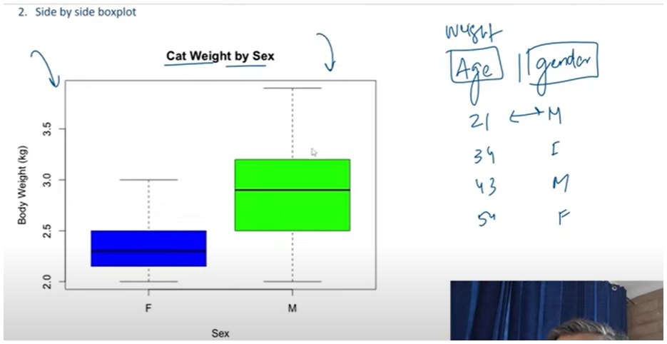
side by side box